Globular cluster luminosity functions

The CASt dataset

Astronomical background

A globular cluster (GC) is a collection of 10⁴-10⁶ ancient stars concentrated into a tight spherical structure structurally distinct from the field population of stars.  Historically, studies of individual stars within GCs were crucial for unravelling the structure and evolution of stars, particularly their red giant phases.  Stellar evolution models show that most GCs were born billions of years ago when the galaxies were young.  Understanding the collective global properties of GCs is now a challenge, as they probably are a small remnant of a once-larger population of clusters, most of which have been disrupted.  Tracing the populations of GCs in nearby galaxies can give clues regarding the different evolution of galaxies including galactic star formation histories (evidenced through GC metallicities), cannabilism (a large galaxy will acquire GCs from smaller merging galaxies), and galactic structure (the GC spatial distribution should reflect the gravitational potential of the galaxy).  GC samples are relatively small; even large galaxies like our Milky Way only have hundreds.   These issues are reviewed in a monograph "Globular Cluster Systems" by K. Ashman & S. Zepf (1998) as well as many papers and conferences.

The distribution of GC luminosities (i.e. the collective brightness of all of its stars)  is known as the globular cluster luminosity function (GCLF).  For unknown reasons, the shape of the GCLF appears to be lognormal in shape with a universal (though with some dependences on covariates such as metallicity) mean and standard deviation.  The peak of the GCLF has thus been used as one of several methods to measure the distances to galaxies.  Detailed study is quite complicated: establishing luminosities from observed brightnesses requires corrections for absorption by interstellar dust; luminosities appear to be statistically linked to metallicities; and halo vs. disk GC populations may systematically differ.  It is also difficult to obtain complete samples of GCs both in other galaxies as surveys are typically "magnitude limited"; i.e. truncated in observed brightness which gives a truncatation in intrinsic luminosity.  A multivariate database for 150 GCs in the Milky Way Galaxy (MWG) is provided by William Harris at http://www.physics.mcmaster.ca/Globular.html. Over 400 Milky Way GCs are known.

Dataset

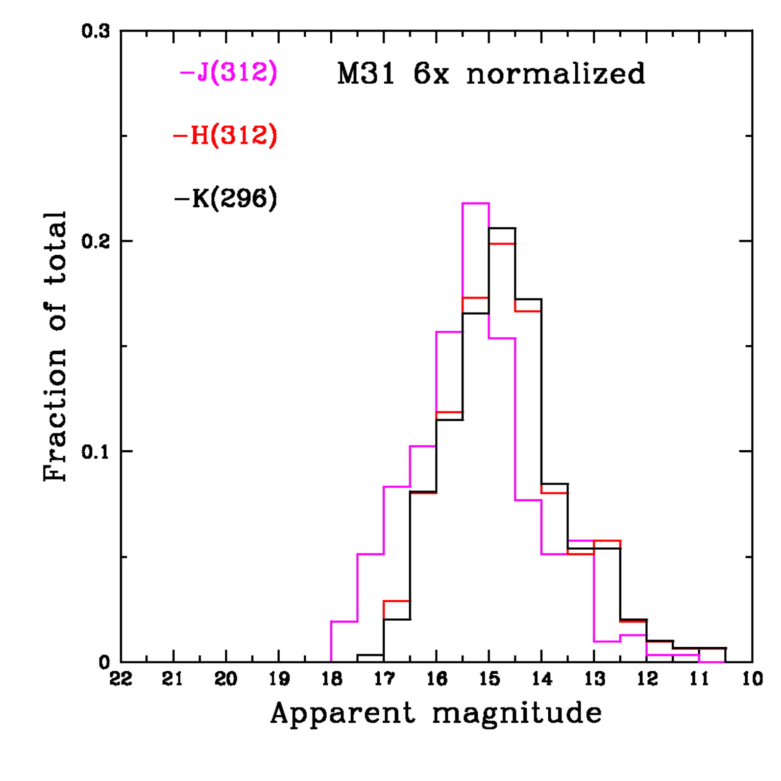
Here we treat the relatively simple univariate datasets of brightnesses for 81 GCs in our MWG and 360 GCs in the nearest large spiral galaxy, the Andromeda Galaxy (M 31). We use the near-infrared K band magnitudes which are less vulnerable to interstellar absorption than visual band magnitudes.  Measurement errors are small and are ignored here.  The columns are: GC name, K-band magnitude.  For the MWG, we give the absolute magnitudes which is an inverted logrithmic unit for intrinsic luminosity). For M 31, we give the apparent magnitude which is offset from absolute magnitude by the "distance modulus", measured to be 24.44 +/- 0.1 for M 31.  In both cases, K band photometry is obtained from the 2MASS All-Sky Survey and is available for only a (biased) subset of the full MWG and M 31 GC populations.

The datasets, figures and numerical results below are obtained from the following paper:

Nearby Spiral Globular Cluster Systems I: Luminosity Functions; Nantais J.B., Huchra J.P., Barmby P., Olsen K.A.G., Jarrett T.H., Astronomical Journal 131, 1416-1425 (2006)

Statistical exercises

• Assuming the MWG is complete and unbiased, fit a normal model.  Test whether the model is valid.
  
• Test whether the M 31 sample is consistent with a normal distribution (black histogram in figure above).  First assume the sample is complete and unbiased.  Second, truncate the sample for magnitudes K>15.5 (the completeness limit of the 2MASS survey) and compute the normal model using maximum likelihood or moment techniques.  See Secker & Harris (Astron J 105, 1358 1993) and "Truncated and Censored Samples" Theory and Applications (Clifford Cohen, 1991) for methdological discussions.
• Apply parametric and nonparametric two sample tests to establish whether the MWG and M 31 GC LFs are consistent with each other.
  
• Calculate the distance modulus of M31 and compare with the value 24.41 +/- 0.1 obtained with Cepheid variable distances.