Introduction to R

Hello, R!

R is a free statistical software. It has many uses including

performing simple calculations (like a very powerful pocket calculator)
making plots (graphs, diagrams etc),
analysing data using ready-made statistical tools (e.g.,, regression),
and above all it is a powerful programming language.

We shall acquaint ourselves with the basics of R in this tutorial.

Starting R

First you must have R installed in your computer. Then typically you have to hunt for an icon like

and double click on it. If everything goes well, you should see a window pop up containing something like this.


R : Copyright 2005, The R Foundation for Statistical Computing
Version 2.1.1  (2005-06-20), ISBN 3-900051-07-0

R is free software and comes with ABSOLUTELY NO WARRANTY.
You are welcome to redistribute it under certain conditions.
Type 'license()' or 'licence()' for distribution details.

  Natural language support but running in an English locale

R is a collaborative project with many contributors.
Type 'contributors()' for more information and
'citation()' on how to cite R or R packages in publications.

Type 'demo()' for some demos, 'help()' for on-line help, or
'help.start()' for a HTML browser interface to help.
Type 'q()' to quit R.

>

The > is the R prompt. You have to type commands in front of this prompt and press the

key on your keyboard.

Simple arithmetics

R may be used like a simple calculator. Type the following command in front of the prompt and hit


2 + 3

Ignore the [1] in the output for the time being. We shall learn its meaning later. Now try


2 / 3

What about the following? Wait! Don't type these all over again.


2 * 3
2 - 3


	Just hit the key of your keyboard to replay the last line. Now use the and cursor keys and the key to make the necessary changes.

Exercise: What does R say to the following?
2/0
Guess what is going to be the result of
2/Inf
and of
Inf/Inf

So now you know about three different types of `numbers' that R can handle: ordinary numbers, infinities, NaN (Not a Number).

Variables

R can work with variables. For example


x = 4

assigns the value 4 to the variable x. This assignment occurs silently, so you do not see any visible effect immediately. To see the value of x type

This is a very important thing to remember:


	To see the value of the variable just type its name and hit .

Let us create a new variable


y = -4

Exercise: Try the following.
x + y x - 2*y x^2 + 1/y
The caret (^) in the last line denotes power.

Exercise: What happens if you type the following?
z-2*x
and what about the next line
X + Y
Well, I should have told you already: R is case sensitive!

Exercise: Can you explain the effect of this?
x = 2*x

Standard functions

R knows most of the standard functions.

Exercise: Try
sin(x) cos(0) sin(pi) #pi is a built-in constant tan(pi/2)

The part of a line after # is called a comment. It is meant for U, the UseR who use R! R does not care about comments.

Exercise: While you are in the mood of using R as a calculator you may also try
exp(1) log(3) log(-3) log(0) log(x-y)
What is the base of the logarithm?

Getting help

R has many many features and it is impossible to keep all its nuances in one's head. So R has an efficient online help system. The next exercise introduces you to this.

Exercise: Suppose that you desperately need logarithm to the base 10. You want to know if R has a ready-made function to compute that. So type
?log
A new window (the help window) will pop up. Do you find what you need?


	Always look up the help of anything that does not seem clear. The technique is to type a question mark followed by the name of the thing you are interested in. All words written like `this` in this tutorial have online help.

Sometimes, you may not know the exact name of the function that you are interested in. Then you can try the help.search function.

Exercise: Can R compute the Gamma function? As your first effort try
Gamma(2)
Oops! Apparently this is not the Gamma function you are looking for. So try
help.search("Gamma")
This will list all the topics that involve Gamma. After some deliberation you can see that ``Special Functions of Mathematics'' matches your need most closely. So type
?Special
Got the information you needed?

Searching for functions with names known only approximately is often frustrating.


	Sometimes it is easier to google the internet than perform `help.search`!

Functions

We can type


sin(1)

to get the value sin 1. Here sin is a standard built-in function. R allows us to create new functions of our own. For example, suppose that some computation requires you to find the value of

f(x) = x/(1-x)

repeatedly. Then we can write function to do this as follows.


f = function(x) x/(1-x)

Now you may type


f(2)
y = 4
f(y)
f(2*y)

Here f is the name of the function. It can be any name of your choice (as long as it does not conflict with names already existing in R).

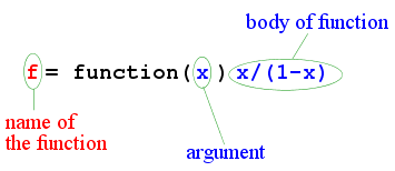Anatomy of an R function

A couple of points are in order here. First, the choice of the name depends completely on you. Second, the name of the argument is also a matter of personal choice. But you must use the same name also inside the body of the function. It is also possible to write functions of more than one variable.

Exercise: Try out the following.
g = function(x,y) (x+2*y)/3 g(1,2) g(2,1)

Exercise: Write a function with name myfun that computes x+2*y/3. Use it to compute 2+2*3/3.

Vectors

So far R appears little more than a sophisticated calculator. But unlike most calculators it can handle vectors, which are basically lists of numbers.


x = c(1,2,4,56)
x

The c function is for concatenating numbers (or variables) into vectors.

Exercise: Try
y = c(x,c(-1,5),x) length(x) length(y)

There are useful methods to create long vectors whose elements are in arithmetic progression:


x = 1:20
4:-10

If the common difference is not 1 or -1 then we can use the seq function


y=seq(2,5,0.3)
y

Exercise: Try the following
1:100
Do you see the meaning of the numbers inside the square brackets?

Exercise: How to create the following vector in R?
1, 1.1, 1.2, , ... 1.9, 2, 5, 5.2, 5.4, ... 9.8, 10
Hint: First make the two parts separately, and then concatenate them.

Working with vectors

Now that we know how to create vectors in R, it is time to use them. There are basically three different types of functions to handle vectors.

those that work entrywise
those that summarise a vector into a few numbers (like finds the sum of all the numbers)
others

Exercise: Most operations that work with numbers act entrywise when applied to vectors. Try this.
x = 1:5 x^2 x+1 2*x sin(x) exp(sqrt(x))

It is very easy to add/subtract/multiply/divide two vectors entry by entry.

Exercise:
x = c(1,2,-3,0) y = c(0,3,4,0) x+y x*y x/y 2*x-3*y

Next we meet some functions that summarises a vector into one or two numbers.

Exercise: Try the following and guess the meanings of commands.
val = c(2,1,-4,4,56,-4,2) sum(val) mean(val) min(val) max(val) range(val)

Exercise: Guess the outcome of
which.min(val) which.max(val)
Check your guess with the online help.

Extracting parts of a vector

If x is vector of length 3 then its entries may be accessed as x[1], x[2] and x[3].


x = c(2,4,-1)
x[1]
x[2]+x[3]
i = 3
x[i]
x[i-1]
x[4]

Note that the counting starts from 1 and proceeds left-to-right. The quantity inside the square brackets is called the subscript or index.


	It is also possible to access multiple entries of a vector by using a subscript that is itself a vector.


x = 3:10
x[1:4]
x[c(2,4,1)]

Exercise: What is the effect of the following?
x = c(10,3,4,1) ind = c(3,2,4,1) #a permutation of 1,2,3,4 x[ind]
This technique is often useful to rearrange a vector.

Exercise: Try the following to find how R interprets negative subscripts.
x = 3:10 x x[-1] x[-c(1,3)]

Subscripting allows us to find one or more entries in a vector if we know the position(s) in the vector. There is a different (and very useful) form of subscripting that allows us to extract entries with some given property.


x = c(100,2,200,4)
x[x>50]

The second line extracts all the entires in x that exceed 50. There are some nifty things that we can achieve using this kind of subscripting. To find the sum of all entries exceeding 50 we can use


sum(x[x>50])

How does this work? If you type


x>50

you will get a vector of TRUEs and FALSEs. A TRUE stands for a case where the entry exceeds 50. When such a True-False vector is used as the subscript only the entries corresponding to the TRUEs are retained. Even that is not all. Internally a TRUE is basically a 1, while a FALSE is a 0. So if you type


sum(x>50)

you will get the number of entries exceeding 50.


	The number of entries satisfying some given property (like ``less than 4'')may be found easily like sum(x<4)

Exercise: If
val = c(1,30,10,24,24,30,10,45)
then what will be the result of the following?
sum(val >= 10 & val <= 40) sum(val > 40 | val < 10) # | means "OR" sum(val == 30) # == means "equal to" sum(val != 24) # != means "not equal to"
Be careful with ==. It is different from =. The former means comparing for equality, while the latter means assignment of a value to a variable.

Exercise: What does
mean(x>50)
denote?

Exercise: Try and interpret the results of the following.
x = c(100,2,200,4) sum(x>=4) mean(x!=2) x==100

Sorting


x = c(2,3,4,5,3,1)
y = sort(x)
y #sorted
x #unchanged

Exercise: Look up the help of the sort function to find out how to sort in decreasing order.

Sometimes we need to order one vector according to another vector.


x = c(2,3,4,5,3,1)
y = c(3,4,1,3,8,9)
ord = order(x)
ord

Notice that ord[1] is the position of the smallest number, ord[2] is the position of the next smallest number, and so on.


x[ord] #same as sort(x)
y[ord] #y sorted according to x

Matrices

R has no direct way to create an arbitrary matrix. You have to first list all the entries of the matrix as a single vector (an m by n matrix will need a vector of length mn) and then fold the vector into a matrix. To create

1 2

3 4

we first list the entries column by column to get

1, 3, 2, 4.

To create the matrix in R:


A = matrix(c(1,3,2,4),nrow=2)
A

The nrow=2 command tells R that the matrix has 2 rows (then R can compute the number of columns by dividing the length of the vector by nrow.) You could have also typed:


A <- matrix(c(1,3,2,4),ncol=2) #<- is same as =
A

to get the same effect. Notice that R folds a vector into a matrix column by column. Sometimes, however, we may need to fold row by row :


A = matrix(c(1,3,2,4),nrow=2,byrow=T)

The T is same as TRUE.

Exercise: Matrix operations in R are more or less straight forward. Try the following.
A = matrix(c(1,3,2,4),ncol=2) B = matrix(2:7,nrow=2) C = matrix(5:2,ncol=2) dim(B) #dimension nrow(B) ncol(B) A+C A-C A%*%C #matrix multiplication A*C #entrywise multiplication A%*%B t(B)

Subscripting a matrix is done much like subscripting a vector, except that for a matrix we need two subscripts. To see the (1,2)-th entry (i.e., the entry in row 1 and column 2) of A type


A[1,2]

Exercise: Try out the following commands to find what they do.
A[1,] B[1,c(2,3)] B[,-1]

Working with rows and columns

Consider the following.


A = matrix(c(1,3,2,4),ncol=2)
sin(A)

Here the sin function applies entrywise. Now suppose that we want to find the sum of each column. So we want to apply the sum function columnwise. We achieve this by using the apply function like this:


apply(A,2,sum)

The 2 above means columnwise. If we need to find the rowwise means we can use


apply(A,1,mean)

Lists

Vectors and matrices in R are two ways to work with a collection of objects. Lists provide a third method. Unlike a vector or a matrix a list can hold different kinds of objects. Thus, one entry in a list may be a number, while the next is a matrix, while a third is a character string (like "Hello R!"). Lists are useful to store different pieces of information about some common entity. The following list, for example, stores details about a student.


x = list(name="Rama", nationality="Indian", height=5.5, marks=c(95,45,80))

We can now extract the different fields of x as


names(x)
x$name
x$hei #abbrevs are OK
x$marks
x$m[2]
x$na #oops!

In the coming tutorials we shall never need to make a list ourselves. But the statistical functions of R usually return the result in the form of lists. So we must know how to unpack a list using the $ symbol as above.


	To see the online help about symbols like `$` type ?"$" Notice the double quotes surrounding the symbol.

Let us see an example of this. Suppose we want to write a function that finds the length, total and mean of a vector. Since the function is returning three different pieces of information we should use lists as follows.


f = function(x) list(len=length(x),total=sum(x),mean=mean(x))

Now we can use it like this:


dat = 1:10
result = f(dat)
names(result)
result$len
result$tot
result$mean

Doing statistics with R

Now that we know R to some extent it is time to put our knowledge to perform some statistics using R. There are basically three ways to do this.

Doing elementary statistical summarisation or plotting of data
Using R as a calculator to compute some formula obtained from some statistics text.
Using the sophisticated statistical tools built into R.

In this first tutorial we shall content ourselves with the first of these three. But first we need to get our data set inside R.

Loading a data set into R

We shall consider part of a data set given in

Distance to the Large Magellanic Cloud: The RR Lyrae Stars Gisella Clementini, Raffaele Gratton, Angela Bragaglia, Eugenio Carretta, Luca Di Fabrizio, and Marcella Maio Astronomical Journal 125, 1309-1329 (2003).

We have slightly doctored the data file to make it compatible with R. The file is called LMC.dat and resides in some folder F:\astro, say. The data set has two columns with the headings Method, Dist and Err. Here are the first few lines of the file:


Method                  Dist        Err
"Cepheids: trig. paral."  18.70     0.16
"Cepheids: MS fitting"    18.55     0.06
"Cepheids: B-W"          18.55     0.10

There are various ways to load the data set. One is to use


LMC = read.table("F:/astro/LMC.dat", header=T)

Note the use of forward slash (/) even if you are working in Windows. Also the header=T tells that the first line of the data file gives the names of the columns. Here we have used the absolute path of the data file. In Unix the absolute path starts with a forward slash (/).


dim(LMC)
names(LMC)
LMC

This object LMC is like a matrix (more precisely it is called a data frame). Each column stores the values of one variable, and each row stores a case. Its main difference with a matrix is that different columns can hold different types of data (for example, the Method column stores character strings, while the other two columns hold numbers). Otherwise, a data frame is really like a matrix. We can find the mean of the Dist variable like this


mean(LMC[,2])
mean(LMC[,"Dist"])

Note that each column of the LMC matrix is a variable, so it is tempting to write


mean(Dist)

but this will not work, since Dist is inside LMC. We can ``bring it out'' by the command


attach(LMC)

Now the command


mean(Dist)

works perfectly. All the values of the Dist variable are different measurements of the same distance. So it is only natural to use the average as an estimate of the true distance. But the Err variable tells us that not all the measurements are equally reliable. So a better estimate might be a weighted mean, where the weights are inversely proportional to the errors. We can use R as a calculator to directly implement this formula:


sum(Dist/Err)/sum(1/Err)

or you may want to be a bit more explicit


wt = 1/Err
sum(Dist*wt)/sum(wt)

Actually there is a smarter way than both of these.


weighted.mean(Dist, 1/Err)

Script files

So far we are using R interactively where we type commands at the prompt and the R executes a line before we type the next line. But sometimes we may want to submit many lines of commands to R at a single go. Then we need to use scripts.


	Use script files to save frequently used command sequences. Script files are also useful for replaying an analysis at a later date.

A script file in R is a text file containing R commands (much as you would type them at the prompt). As an example, open a text editor (e.g., notepad in Windows, or gedit in Linux). Avoid fancy editors like MSWord. Create a file called, say, test.r containing the following lines.


x = seq(0,10,0.1)
y = sin(x)
plot(x,y,ty="l") #guess what this line does!

Save the file in some folder (say F:/astro). In order to make R execute this script type


source("F:/astro/test.r")

If your script has any mistake in it then R will produce error messages at this point. Otherwise, it will execute your script.

The variables x and y created inside the command file are available for use from the prompt now. For example, you can check the value of x by simply typing its name at the prompt.

Commands inside a script file are executed pretty much like commands typed at the prompt. One important difference is that in order to print the value of a variable x on the screen you have to write


print(x)

Merely writing

on a line by itself will not do inside a script file.


	Printing results of the intermediate steps using `print` from inside a script file is a good way to debug R scripts.