Testing and Estimation

A simple example

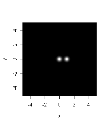
Consider the computer-generated picture below which is supposed to mimic a photograph taken by a low resolution telescope. Is it reasonable to say that there are two distinct stars in the picture?

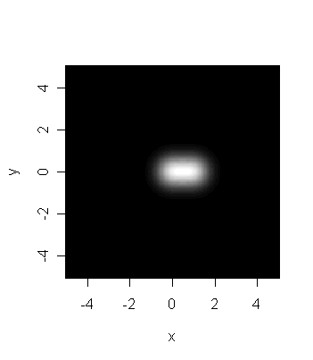
The next image is obtained by reducing the resolution of the telescope. Each star is now more blurred. Indeed, their distance in the picture is almost overwhelmed in the blur, and they appear to be an elongated blur caused by a single star.

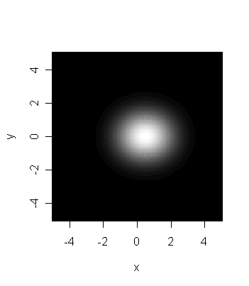
The last picture is is of the same two stars taken through a very low resolution telescope. Based on this image alone there is just no reason to believe that we are seeing two stars.

What we did just now is an informal version of a statistical test of hypothesis. Each time we tried to answer the question ``Are there two stars or one?" based on a blurry picture. The two possibilities

``There is just one star'' as opposed to ``There are two stars''

are called two hypotheses. The simpler of the two gets the name null hypothesis while the other is called the alternative hypothesis. Here we shall take the first one as the null, and the second one as the alternative hypothesis.

The blurry picture we use to make a decision is called the statistical data (which always contains random errors in the form of blur/noise). Notice how our final verdict changes with the amount of noise present in the data.

Let us follow the thought process that led us to a conclusion based on the first picture. We first mentally made a note of the amount of blur. Next we imagined the centres of the bright blobs. If there are two stars then the are most likely to be here. Now we compare the distance between these centres and the amount of blur present. If the distance seems too small compared to the blur then we pass off the entire bundle as a single star.

This is precisely the idea behind most statistical tests. We shall see this for the case of the two sample t-test.

Do Hyades stars differ in colour from the rest?

Recall in the Hipparcos data set we had 92 Hyades stars and 2586 non-Hyades stars. We want to test the null hypothesis

``The Hyades stars have the same colour as the non-Hyades stars''

versus the alternative hypothesis

``They have different colours.''

First let us get hold of the data for both the groups.


source("hyad.r")
colour = B.V
H = colour[HyadFilter]
nH = colour[!HyadFilter & !is.na(colour)]
m = length(H)
n = length(nH)

In the definition of nH above, we needed to exclude the NA values. H is a list of m numbers and

nH

is a list of n numbers.

First we shall make an estimate of the ``blur'' present in the data. For this we shall compute the pooled estimate of standard deviation.


blur.H = var(H)
blur.nH = var(nH)
blur.pool = ((m-1)*var(H) + (n-1)*var(nH))/(m+n-2)

Next we shall find the difference of the two means:


meanDiff = mean(H)-mean(nH)

Finally we have to compare the difference with the blur. One way is to form their ratio.


(meanDiff/sqrt(blur.pool))/sqrt(1/m + 1/n)

This last factor (which is a constant) is there only for technical reasons (you may think of it as a special constant to make the ``units match'').

The important question now is ``Is this ratio small or large?'' For the image example we provided a subjective answer. But in statistics we have an objective way to proceed. Before we see that let us quickly learn a one-line shortcut to compute the above ratio using the t.test function.


t.test(H,nH,var.eq=T) #we shall explain the "var.eq" soon

Do you see the ratio in the output? Also this output tells us whether the ratio is to be considered small or large. It does so in a somewhat diplomatic way using a number called the p-value. Here the p-value is near 0, meaning

if the colours were really the same then then chance of observing a ratio this large (or larger) is almost 0.

Typically, if the p-value is smaller than 0.05 then we reject the null hypothesis. So we conclude that the mean of the colour of the Hyades stars is indeed different from that of the rest.


	A rule of thumb: For any statistical test (not just t-test) accept the null hypothesis if and only if the p-value is above 0.05. Such a test fails to recognise a true null hypothesis at most 5% of the time.

The var.eq=T option means we are assuming that the colours of the Hyades and non-Hyades stars have more or less the same variance. If we do not want to make this assumption, we should simply write


t.test(H,nH)


	Use `t.test` for comparing means.

Chi-squared tests for categorical data

Suppose that you are to summarise the result of a public examination. It is not a reasonable to report the grades obtained by each and every student in a summary report. Instead, we break the range of marks into categories like first division, second division, third division, failed etc. and then report the numbers of students in each category. This gives an overall idea about the distribution of grades.

The cut function in R does precisely this.


bvcat = cut(colour, breaks=c(-Inf,0.5,0.75,1,Inf))

Here we have broken the range of values of the B.V variable into 4 categories:

(-Inf, 0.5], (0.5, 0.75], (0.75, 1] and (1,Inf).

The result (stored in bvcat) is a vector that records the category in which each star falls.


bvcat 
table(bvcat)
plot(bvcat)

It is possible to tabulate this information for Hyades and non-Hyades stars in the same table.


table(bvcat,HyadFilter)

To perform a chi-squared test of the null hypothesis that the true population proportions falling in the four categories are the same for both the Hyades and non-Hyades stars, use the chisq.test function:


chisq.test(bvcat,HyadFilter)

Since we already know these two groups differ with respect to the B.V variable, the result of this test is not too surprising. But it does give a qualitatively different way to compare these two distributions than simply comparing their means.

The test above is usually called a chi-squared test of homogeneity. If we observe only one sample, but we wish to test whether the categories occur in some pre-specified proportions, a similar test (and the same R function) may be applied. In this case, the test is usually called the chi-squared test of goodness-of-fit. We shall see an example of this next.

Consider once again the Hipparcos data. We want to know if the stars in the Hipparcos survey come equally from all corners of the sky. In fact, we shall focus our attention only on the RA values. First we shall break the range of RA into 20 equal intervals (each of width 18 degrees), and find how many stars fall in each bin.


count = table(cut(RA,breaks=seq(0,360,len=20)))
chisq.test(count)

Kolmogorov-Smirnov Test

There is yet another way (a better way in many situations) to perform the same test. This is called the Kolmogorov-Smirnov test.


ks.test(RA,"punif",0,360)

Here punif is the name of the distribution with which we are comparing the data. punif denoted the uniform distribution, the range being from 0 to 360. Thus, here we are testing if RA is taking all values from 0 to 360 with equal likelihood, or are some values being taken more or less frequently.

The Kolmogorov-Smirnov test has the advantage that we do not need to group the data into categories as for the chi-squared test.


	Use `chisq.test` and `ks.test` for comparing distributions.

Estimation

Finding (or, rather, guessing about) the unknown based on approximate information (data) is the aim of statistics. Testing hypotheses is one aspect of it where we seek to answer yes-no questions about the unknown. The problem of estimation is about guessing the values of unknown quantities.

There are many methods of estimation, but most start off with a statistical model of the data. This is a statement of how the observed data set is (probabilistically) linked with the unknown quantity of interest.

For example, if I am asked to estimate p based on the data

Head, Head, Head, Tail, Tail, Head, Head, Tail, Head, Tail, Tail, Head

then I cannot make head-or-tail of the question. I need to link this data set with p through a statement like

A coin with probability p was tossed 12 times and the data set was the result.

This is a statistical model for the data. Now the problem of estimating p from the data looks like a meaningful one.


	Statistical models provide the link between the observed data and the unknown reality. They are indispensable in any statistical analysis. Misspecification or over-simplification of the statistical model is the most frequent cause behind misuse of statistics.

Estimation using R

You might be thinking that R has some in-built tool that can solve all estimation problems. Well, there isn't. In fact, due to the tremendous diversity among statistical models and estimation methods no statistical software can have tools to cope with all estimation problems. R tackles estimation in three major ways.

Many books/articles give formulae to estimate various quantities. You may use R as a calculator to implement them. With enough theoretical background you may be able to come up with your own formulae that R will happily compute for you.
Sometimes estimation problems lead to complicated equations. R can solve such equations for you numerically.
For some frequently used statistical methods (like regression or time series analysis) R has the estimation methods built into it.

To see estimation in action let us load the Hipparcos data set.


hip = read.table("HIP.dat",head=T)
attach(hip)
Vmag

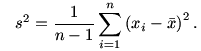
If we assume the statistical model that the Vmag variable has a normal distribution with unknown mean μ and unknown variance σ² then it is known from the literature that a good estimator of μ is and a 95% confidence interval is

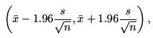
where

This means that the true value of μ will lie in this interval with 95% chance. You may think of μ as a peg on the wall and the confidence interval as a hoop thrown at it. Then the hoop will miss the peg in only about 5% of the cases.

Exercise: Find the estimate and confidence interval for μ based on the observed values of Vmag using R as a calculator.

Next we shall see a less trivial example. The data set comes from NASA's Swift satellite. The statistical problem at hand is modeling the X-ray afterglow of gamma ray bursts. First, read in the dataset:


dat = read.table("GRB.dat",head=T)
flux = dat[,2]

Suppose that it is known that the flux variable has an Exponential distribution. This means that its density function is of the form

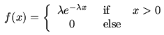
Here λ is a parameter, which must be positive. To get a feel of the density function let us plot it for different values of λ


x = seq(0,200,.1)
y = dexp(x,1)
plot(x,y,ty="l")

Now let us look at the histogram of the observed flux values.


hist(flux)

The problem is estimating λ based on the data may be considered as finding a value of λ such that the the density is as close as possible to the histogram.

We shall first try to achieve this interactively.


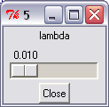
source("interact.r")

This should open a tiny window as shown below with a slider and a button in it.

Screenshot of the tiny window

Move the slider to see how the density curve moves over the histogram. Choose a position of the slider for which the density curve appears to be a good approximation.

Exercise: It is known from the theory of Exponential distribution that the Maximum Likelihood Estimate (MLE) of λ is the reciprocal of the sample mean

Compute this estimate using R and store it in a variable called lambdaHat.
Draw the density curve on top of the histogram using the following commands.
y = dexp(x,lambdaHat) lines(x,y,col="blue")