Simulation and Bootstrapping

Simulation

Many people think of a coin toss when they think about randomness. While everything in nature is random, a coin toss has the extra quality of being a completely known process. We do not know what the outcome of the next coin is going to be, but we know the average behavior quite well, viz., the outcome will be either a Head or a Tail, each of which is equally likely. It is this perfect knowledge that leads us to use a coin toss when making a fair decision.

A coin toss is a random mechanism that we can repeat at our will to produce random quantities with a known behavior. Another such a device is a die. But such practical devices used to be limited in number and scope before the advent of high speed computers.

A remarkable fact about computers is that they can be instructed to produce random quantities whose general behavior is completely under control. We can, for example make the computer toss a coin with exactly a specified amount of bias for Head! We can turn the computer easily into a 100-faced die, something that is almost to construct in practice. In fact, computers can be made to perform more exotic (as well more useful) random computations that have started to play a dominant role in statistics. In this last tutorial we shall take a look at these.

Putting it in perspective

Man has devised various techniques to deal with chance. These may be classified into roughly three categories:

Wait and see: Here we patiently wait until the end of the activity. This time-honored method remains the most frequently used one even today. Who can deny the usefulness of observing the sky carefully to learn about the random patterns? However, learning by just trial-and-error may prove too expensive. When we want to design a space station to maximize its chance of capturing some rare phenomenon, it would prove it bit too costly to simply rely on trial and error!
Use probability models: Often we have enough information (theoretical and/or based on prior observations) about the mechanism underlying a random phenomenon. For example, if a careful scrutiny of a die does not reveal any difference between the faces of a die, one may assume that the die is fair. Such information can be expressed as a probability distribution:
The outcome X can take values 1,...,6 each with equal probability (taken to be 1/6 to keep the sum 1).
Using this mathematical formulation of our knowledge about the random phenomenon we can now analyze the distribution mathematically. For example, consider the following gambling game
A die is rolled, and the casino owner gives you Re 1 for each point shown. For example, you get Rs 6 if the die shows a 6. How much will you get on average per roll if you play this game 10000 times?
The brute force approach is to really play it 10000 times, and then divide the total amount by 10000. A smarter way is to use the probability distribution of the die. We know that on average we get 1 about 1/6 of the times, 2 about 1/6 of the times and so on. So on an average we shall get
(1+2+3+4+5+6)/6 = 3.5
per roll. Here the math turned out to be simple. But in more realistic models the math is often too tough to handle even with a computer!
Simulate probability models: Here also we start with a model. But instead of dealing with it mathematically, we make the computer to perform (or simulate) the random experiment following the model. This is possible because computers can generate random numbers

Actually computers generate only pseudo-random numbers. These are not random but only behave like random numbers. However, we shall disregard the difference here.

Now it is just like the "wait and see" strategy, except that we do not have to wait long, since computers can perform many repetitions of a random experiment very fast. Also, no real monetary loss is involved.

Let us see the third approach in action for the gambling example before we move on to more serious applications.

values = 1:6 #the possible values
sample(values, 10, replace=T)

This last line asks R to sample 10 numbers from the vector values. The ``replace=T'' allows the same number to occur multiple times. Run the last line repeatedly to see that how the output changes randomly. Now to solve the problem use

money = sample(values, 10000, replace=T)
avg = mean(money)
avg

This mean is indeed pretty close to the theoretical 3.5. But will it always be the case? After all it is random game. So it is a good idea to repeat the above simulation a number of times, say, 100 times. The blue lines below are as before. But these are now enveloped in some extra lines (shown in bold). This is an example of a for loop.


avgList = c() #an empty vector
for(i in 1:100) {
   money = sample(values, 10000, replace=T)
   avg = mean(money)
   avgList = c(avgList,avg) #add avg to avgList
}

mean(avgList)
var(avgList)

To repeat some commands for a fixed number of times (say 200) in R you put the commands inside a for loop like this


for(i in 1:200) {
   #Your commands
   #go here
}

For example, you may try

for(i in 1:5) {
   print("hello")
}

Simulating from a distribution

The fundamental concept behind the above technique is that R can ``roll a die'' or, rather, ``simulate a die''. Statistically this means generating a random number from among the values 1,...,6 with probabilities 1/6 each. This is by no means the only distribution R can generate numbers from. We can for example, generate a random number from the Uniform(0,1) distribution. Such a number can take any value between 0 and 1, each value being equally likely. Let us generate 100 such numbers.

data = runif(1000, min=0, max=1)
hist(data)

R has many probability distributions built into it, and it has ready-made functions (like runif) to generate data from them. The functions all share a common naming pattern. They start with the letter `r' followed by an acronym for the distribution. Here are some examples.

data = rnorm(1000, mean=1, sd=2) #Normal(1,2)
hist(data)
data = rpois(1000, lambda=1) #Poisson(1)
hist(data)
data = rexp(1000, rate=2) #Exponential with mean 1/2
hist(data)

Two realistic examples

An imperfect particle counter

A huge radio active source emits particles at random time points. A particle detector is detecting them. However, the detector is imperfect and gets ``jammed'' for 1 sec every time a particle hits it. No further particles can be detected within this period. After the 1 sec is over, the detector again starts functioning normally. We want to know the fraction of particles that the detector is missing. Since this fraction may depend on the rate at which the source emits particles we want to get a plot like the following:

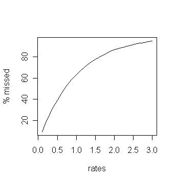Want a plot like this

Random emission of particles from a huge radio active source is well-studied process. A popular model is to assume that the time gaps between successive emissions are independent and have Exponential distributions.

gaps = rexp(999,rate=1)

The question now is to determine which of the particles will fail to be detected. A particle is missed if it comes within 1 sec of its predecessor. So the number of missed particles is precisely the number of gaps that are below 1.

miss = sum(gaps < 1)
miss

Now we want to repeat this experiment a number of times, say 50 times.


missList = c()
for(i in 1:50) {
   gaps = rexp(999,rate=1)
   miss = sum(gaps < 1)
   missList = c(missList,miss)
}
mean(missList)
var(missList)

All these are done for rate = 1. For other rates we need to repeat the entire process afresh. So we shall use yet another for loop.


rates = seq(0.1,3,0.1)
mnList = c()
vrList = c()
for(lambda in rates) {
   missList = c()
   for(i in 1:50) {
      gaps = rexp(1000,rate=lambda)
      miss = sum(gaps < 1)
      missList = c(missList,miss)
   }

   mn = mean(missList)
   vr = var(missList)
   mnList = c(mnList,mn)
   vrList = c(vrList, vr)
}

Now we can finally make the plot.

plot(rates,mnList/10,ty="l",ylab="% missed")

We shall throw in two error bars for a good measure.

up = mnList + 2*sqrt(vrList)
lo = mnList - 2*sqrt(vrList)

lines(rates,up/10,col="red")
lines(rates,lo/10,col="blue")

Exercise: (This exercise is difficult) We can estimate the actual rate from the hitting times of the particles if the counter were perfect. The formula is to take the reciprocal of the average of the gaps. But if we apply the same formula for the imperfect counter, then we may get a wrong estimate of the true rate. We want to make a correction graph that may be used to correct the under estimate. Explain why the following R program achieves this. You will need to look up the online help of cumsum and diff.
rates = seq(0.1,3,0.1) avgUnderEst = c() for(lambda in rates) { underEst = c() for(i in 1:50) { gaps = rexp(1000,rate=lambda) hits = cumsum(gaps) obsHits = c(hits[1], hits[gaps>1]) obsGaps = diff(obsHits) underEst = c(underEst,1/mean(obsGaps)) } avgUnderEst = c(avgUnderEst,mean(underEst)) } plot(avgUnderEst,rates,ty="l")
Can you interpret the plot?

Simulating a galaxy

A galaxy is not a single homogeneous body and so it has different mass densities at different points. When we say that the mass density of a galaxy at a point (x,y,z) is f(x,y,z) we mean that for any region R in that galaxy the chance of detecting a body is

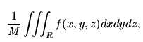
where M is the total mass of the galaxy.

There are various models that specify different forms for f. Many of these consider the galaxy to be confined in some 2D plane, so that the density may be written as f(x,y). The typical process for simulating a galaxy has two components:

First we simulate the initial state of the galaxy from some probability model.
Next, we let it evolve deterministically following appropriate laws of motion.

Such simulations are extremely computation intensive. We shall therefore confine ourselves to a very simple situation. To keep life simple we shall assume that the x and y-coordinates of the stars are independent normal random variables. We shall work with just 500 stars of equal masses. (It is easy to allow random masses, but in our simple implementation the simulation would then take awfully long to run!) Each star initially has tangential velocity proportional to the distance from the center.

x = rnorm(500,sd=4)
y = rnorm(500,sd=4)
vx = -0.5*y
vy = 0.5*x

Let us plot the initial stage of our galaxy.

oldpar = par(bg="black") #we want black background
plot(x,y,pch=".",col="white") #and white stars
par(oldpar) #restore the default (black on white)

This does not look much like a galaxy. We have to let it evolve over time. This basically means solving an n-body problem numerically. A popular method is the Hut-Barnes algorithm. But we shall apply Newton's laws using R in a brute force (and slow) way. The commands are in the script file newton.r.

source("newton.r")

Here we shall perform the simulation for 100 time steps, updating the picture of the galaxy every 10 steps. With only 500 points it is difficult to see much pattern, but still one may see spiral tentacles forming.

The simulation here is admittedly very crude and inefficient. If you are interested, you may see more realistic examples (with references) at this website.

Bootstrapping

So far we are simulating from completely specified distributions. But suppose that someone gives some data and asks us to simulate from whatever is the distribution of the data. Since we do not have the distribution itself we cannot apply the above methods directly.

However, as it happens, there is an approximate way out that is simple to implement in R. Let us first see it using an artificial example.

Suppose someone has some data that was originally generated from N(0,1) distribution.

origData = rnorm(1000,mean=0,sd=1)

Then we shall simply resample from this data set.

newData = sample(origData,500, replace=T)

This is called (one form of) bootstrapping.

It is instructive to compare this with the true distribution.

hist(newData,prob=T)
x = seq(-3,3,0.1)
lines(x,dnorm(x))

Now let us apply this on some real data.

hip = read.table("HIP.dat", header = TRUE, fill = TRUE)
attach(hip)

We shall consider the Vmag variable. We want to generate 10 new values from its distribution (which is unknown to us).

newVmag = sample(Vmag,10,replace=T)

Well, that was easily done, but the question is

What in the universe does this newVmag mean?

Does this mean we have generated 10 new galaxies? How can that be when we are just re-using the old values?

Common sense, please!

First let us beware of the following mistaken notion.


	Mistaken notion: Bootstrapping is a way to increase the sample size without any extra real sampling.

If that were true, you could just keep on generating further samples from existing data and get away by pretending that they are new galaxies. Well, common sense tells us that this cannot be true.


	Great lesson: Never place statistics above common sense.

By repeatedly picking from the already available sample we are not adding anything to the information. In particular, if the original sample presents a biased view of the underlying population, then none of the resamples can cure that distortion.

Why then should we do bootstrapping at all?

The next example explains why this is useful.

Astronomical data sets are often riddled with outliers (values that are far from the rest). To get rid of such outliers one sometimes ignores a few of the extreme values. One such method is the trimmed mean.

x = c(1,2,3,4,5,6,100,7,8,9)
mean(x)
mean(x,trim=0.1) #ignore the extreme 10% points in BOTH ends
mean(x[x!=1 & x!=100])

We shall compute 10%-trimmed mean of Vmag from the Hipparcos data set.

hip = read.table("HIP.dat", header = TRUE, fill = TRUE)
attach(hip)
mean(Vmag,trim=0.1)

We want to estimate the standard error of this estimate. For ordinary mean we had a simple formula, but unfortunately such a simple formula does not exist for the trimmed mean. So we shall use bootstrap here as follows. We shall generate 100 resamples each of same size as the original sample.

trmean = c()
for(i in 1:100) {
   resamp = sample(Vmag,length(Vmag),replace=T)
   trmean = c(trmean,mean(resamp,trim=0.1))
}
sd(trmean)


	Bootstrapping is such a popular statistical technique that R has a package called `boot` to perform bootstrapping.

Permutation test

Here is a variation of the same theme: resampling i.e., randomly sampling from the original sample and pretending that it is a new sample.

The situation that we are discussing next involves two samples, say, the Hyades and the non-Hyades stars. Suppose that we want to see if the their medians colors are different or not. (By this, as usual, we mean to test if the medians of the distributions underlying the two samples are same or not.) Here we shall assume that the shapes of the two distributions are the same. Since the samples are pretty large, it is reasonable to look at the differences of the medians of the two samples.

source("hyad.r")
colH = B.V[HyadFilter]
colnH = B.V[!HyadFilter & !is.na(B.V)]
m = length(colH)
n = length(colnH)
median(colH)-median(colnH)

If the population medians are the same, then we should expect this difference to be near zero, as well. So if this difference is too large, then we have reason to suspect that the underlying distributions have different medians. The question therefore is how large is ``too large"?

Sometimes statistical theory dictates a rule to decide this. But more often there is no theory to help. Then permutation tests provide an easy way out.

Imagine first what happens if the medians are the same. Then the two underlying distributions are actually the same (since their shapes already match by assumption). So the two samples together is basically like a single large sample from this common distribution. If this is the case, calling a Hyades star as non-Hyades (or vice versa) would really not make any difference.

So we shall mix up all stars together, and then pick any m of them and call them Hyades, while the remaining n would be labeled nonHyades. This should be as good as the original sample if the two distributions are indeed the same.

pool = c(colH,colnH)
mixed = sample(pool) # sample generates a random permutation
newH = mixed[1:m]
newnH = mixed[(m+1):n]
median(newH) - median(newnH)

If the two distributions were really the same then this new difference should be close to the difference based on the original data.

Of course, this apparently takes us back to the original question: how close is ``close enough"? But now it is easier to answer since we can repeat this random mixing many times.

pool = c(colH,colnH)
d = c()

for(i in 1:1000) {
   mixed = sample(pool)
   newH = mixed[1:m]
   newnH = mixed[(m+1):n]
   newDiff = median(newH) - median(newnH)
   d = c(d,newDiff)
}

Now that we have 1000 values of how the typical difference should look like if the distributions were the same, we can see where our original difference lies w.r.t. these values. First let us make a histogram of the typical values:

hist(d)

Well, the original value seems quite far from the range of typical values, right?

One way to make this idea precise is to compute the p-value, which is defined as the chance of observing a difference even more extreme than the original value. Here ``more extreme" means ``larger in absolute value".

orig = median(colH)-median(colnH)
sum(abs(d)>=abs(orig))/1000

A p-value smaller than 0.05, say, strongly indicates that the medians of the distributions are not the same.