Testing and Estimation
A simple example
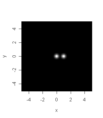
Consider the computer-generated picture below which is supposed to
mimic a
photograph taken by a low resolution telescope. Is it reasonable
to say that there are two distinct stars in the picture?
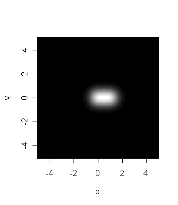
The next image is obtained by reducing the resolution of the
telescope. Each star is now more blurred. Indeed, their distance
in the picture is almost overwhelmed in the blur, and they appear
to be an elongated blur caused by a single star.
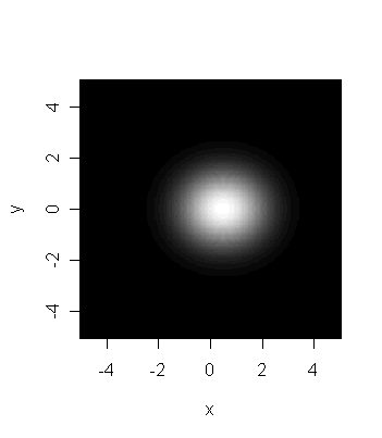
The last picture is is of the same two stars taken through a very
low resolution telescope. Based on this image alone there
is just no reason to believe that we are seeing two stars.
What we did just now is an informal version of a statistical test
of hypothesis. Each time we tried to answer the question ``Are
there two
stars or one?" based on a blurry picture. The two possibilities
``There is just one star'' as opposed to
``There are two stars''
are called two hypotheses. The simpler of the two gets the
name null hypothesis while the other is called the
alternative hypothesis. Here we shall take the first one
as the null, and the second one as the alternative hypothesis.
The blurry picture we use to make a decision is called the
statistical data (which always contains random
errors in the form of blur/noise). Notice how our final verdict
changes with the
amount of noise present in the data.
Let us follow the thought process that led us to a conclusion
based on the first picture. We first mentally made a note of the
amount
of blur. Next we imagined the centers of the bright blobs. If
there are two stars then the are most likely to be here. Now we
compare the distance between these centers and the amount of
blur present. If the distance seems too small compared to the
blur then we pass off the entire bundle as a single star.
This is precisely the idea behind most statistical tests. We
shall see this for the case of the two sample t-test.
Do Hyades stars differ in color from the rest?
Recall in the Hipparcos data set we had 92 Hyades stars and 2586
non-Hyades stars. We want to test the null hypothesis
``The Hyades stars have the same color as the non-Hyades stars''
versus the alternative hypothesis
``They have different colors.''
First let us get hold of the data for both the groups. For this
we shall use the little script we had saved earlier. This script
is going to load the entire Hipparcos data set, and extract the
Hyades stars. So you must make sure that both
HIP.dat and hyad.r are saved on your
desktop. Right-click on the links in the last line, choose
"Save link as..." or "Save target as..." (and be careful that the
files do not get saved a .txt files). Then you must navigate R to
the desktop. The simplest way to achieve this is to use the File
> Change dir... menu item. This will open a pop up like this:
 |
| Changing directory in R (Windows version) |
Click on Desktop, and then OK.
source("hyad.r")
color = B.V
H = color[HyadFilter]
nH = color[!HyadFilter & !is.na(color)]
m = length(H)
n = length(nH)
In the definition of nH above, we needed to exclude the NA
values. H is a list of m numbers and nH
is a list of n numbers.
First we shall make an estimate of the ``blur'' present in the
data. For this we shall compute the pooled estimate of standard
deviation.
blur.H = var(H)
blur.nH = var(nH)
blur.pool = ((m-1)*var(H) + (n-1)*var(nH))/(m+n-2)
Next we shall find the difference of the two means:
meanDiff = mean(H)-mean(nH)
Finally we have to compare the difference with the blur. One way
is to form their ratio.
(meanDiff/sqrt(blur.pool))/sqrt(1/m + 1/n)
This last factor (which is a constant) is there only for
technical reasons (you may think of it as a special constant to
make the ``units match'').
The important question now is ``Is this ratio small or large?''
For the image example we provided a subjective answer. But in
statistics we have an objective way to proceed. Before we see
that let us quickly learn a one-line shortcut to compute the above
ratio using the t.test function.
t.test(H,nH,var.eq=T) #we shall explain the "var.eq" soon
Do you see the ratio in the output? Also this output tells us
whether the ratio is to be considered small or large. It does so
in a somewhat diplomatic way using a number called the
p-value. Here the p-value is near 0, meaning
if the colors were really the same then then chance of observing
a ratio this large (or larger) is almost 0.
Typically, if the p-value is smaller than 0.05 then we reject the
null hypothesis. So we conclude that the mean of the color of
the Hyades
stars is indeed different from that of the rest.
 |
 |  |  |
|
A rule of thumb: For any statistical test (not just
t-test) accept the null hypothesis if and only if the
p-value is above 0.05. Such a test fails to recognize a true
null hypothesis at most 5% of the time.
| |
 | |  |
|
The var.eq=T option means we are assuming that the
colors of the Hyades and non-Hyades stars have more or less the
same variance. If we do not want to make this assumption, we
should simply write
t.test(H,nH)
|
| | |
|
Remember: t.test is for comparing means.
| |
| | |
|
Chi-squared tests for categorical data
Suppose that you are to summarize the result of a public
examination. It is not a reasonable to report the grades obtained
by each and every student in a summary report. Instead, we break
the range of grades into categories like A,B,C etc and
then report the numbers
of students in each category. This gives an overall idea about
the distribution of grades.
The cut function in R does precisely this.
bvcat = cut(color, breaks=c(-Inf,0.5,0.75,1,Inf))
Here we have broken the range of values of the B.V
variable into 4 categories:
(-Inf, 0.5], (0.5, 0.75], (0.75, 1] and (1,Inf).
The result (stored in bvcat) is a vector that
records the category in which each star falls.
bvcat
table(bvcat)
plot(bvcat)
It is possible to tabulate this information for Hyades and
non-Hyades stars in the same table.
table(bvcat,HyadFilter)
To perform a chi-squared test of the null hypothesis that the
true population proportions falling in the four categories are
the same for both the Hyades and non-Hyades stars, use the
chisq.test function:
chisq.test(bvcat,HyadFilter)
Since we already know these two groups differ with respect to the
B.V variable, the result of this test is not too
surprising. But
it does give a qualitatively different way to compare these two
distributions than simply comparing their means.
The test above is usually called a chi-squared test of
homogeneity. If we observe only one sample, but we wish to test
whether the categories occur in some pre-specified proportions, a
similar test (and the same R function) may be applied. In this
case, the test is usually called the chi-squared test of
goodness-of-fit. We shall see an example of this next.
Consider once again the Hipparcos data.
We want to know if the stars in the
Hipparcos survey come equally from all corners of the sky. In
fact, we shall focus our attention only on the RA
values.
First we shall break the range of RA into 20 equal intervals (each of
width 18 degrees), and find how many stars fall in each bin.
count = table(cut(RA,breaks=seq(0,360,len=20)))
chisq.test(count)
Kolmogorov-Smirnov Test
There is yet another way (a better way in many situations) to
perform the same test. This is called the Kolmogorov-Smirnov
test.
ks.test(RA,"punif",0,360)
Here punif is the name of the distribution with
which we are comparing the data. punif denoted the
uniform distribution, the range being from 0 to 360. Thus, here
we are testing if RA is taking all values from 0
to 360 with equal likelihood, or are some values being taken more
or less frequently.
The Kolmogorov-Smirnov test has the advantage that we do not need
to group the data into
categories as for the chi-squared test.
|
| | |
|
Remember: chisq.test and ks.test are for comparing
distributions.
| |
| | |
|
Estimation
Finding (or, rather, guessing about) the unknown based on
approximate information (data) is the aim of statistics. Testing
hypotheses is
one aspect of it where we seek to answer yes-no questions about
the unknown. The problem of estimation is about guessing the
values of unknown quantities.
There are many methods of estimation, but most start off with a
statistical model of the data. This is a statement of how
the observed data set is (probabilistically) linked with the
unknown quantity of interest.
For example, if I am asked to estimate p based on the data
Head, Head, Head, Tail, Tail, Head, Head, Tail, Head, Tail, Tail, Head
then I cannot make head-or-tail of the question. I need to link
this data set with p through a statement like
A coin with probability p was tossed 12 times and the data
set was the result.
This is a statistical model for the data. Now the problem of
estimating p from the data looks like a meaningful one.
|
| | |
|
Statistical models provide the link between the observed data and
the unknown reality. They are indispensable in any statistical
analysis. Misspecification or over-simplification of the
statistical model is the most frequent cause behind misuse of
statistics.
| |
| | |
|
Estimation using R
You might be thinking that R has some in-built tool that can
solve all estimation problems. Well, there isn't. In fact, due to
the tremendous diversity among statistical models and estimation
methods no statistical software can have tools to cope
with all estimation problems. R tackles estimation
in three major ways.
- Many books/articles give formulas to estimate various
quantities. You may use R as a calculator to implement them.
With enough theoretical background you may be able to come up
with your own formulas that R will happily compute for you.
- Sometimes estimation problems lead to complicated
equations. R can solve such equations for you numerically.
- For some frequently used statistical methods (like
regression or time series analysis) R has the estimation methods
built into it.
To see estimation in action let us load the Hipparcos data set.
hip = read.table("HIP.dat", header = TRUE, fill = TRUE)
attach(hip)
Vmag
If we assume the statistical model that the Vmag
variable has a normal distribution with unknown mean μ and
unknown variance σ2 then it is known from the literature
that a good estimator of μ is  and a
95% confidence interval is
and a
95% confidence interval is
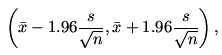
where
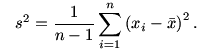
This means that the true value of μ will lie in this
interval with 95% chance. You may think of μ as
a peg on the wall and the confidence interval as a hoop thrown at
it. Then the hoop will miss the peg in only about 5% of
the cases.
| Exercise:
Find the estimate and confidence interval for μ based
on the observed values of Vmag using R as a calculator.
|
Next we shall see a less trivial example.
The data set comes from NASA's Swift satellite. The statistical
problem at hand is modeling the X-ray afterglow of gamma ray
bursts. First, read in the dataset GRB.dat
(right-click, save on your desktop, without any .txt extension).
dat = read.table("GRB.dat",head=T)
flux = dat[,2]
Suppose that it is known that the flux variable has
an Exponential distribution. This means that its density function
is of the form
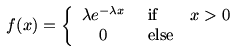
Here λ is a parameter, which must be positive. To
get a feel of the density function let us plot it for different
values of λ
x = seq(0,200,.1)
y = dexp(x,1)
plot(x,y,ty="l")
Now let us look at the histogram of the observed
flux values.
hist(flux)
The
problem is estimating λ based on the data may be
considered as finding a value of λ such that the
the density is as close as possible to the histogram.
We shall first try to achieve this interactively. For this you
need to download interact.r on your desktop first.
source("interact.r")
This should open a tiny window as shown below with a slider and a
button in
it.
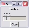 |
| Screenshot of the tiny window |
Move the slider to see how the density curve moves over the
histogram. Choose a position of the slider for which the density
curve appears to be a good approximation.
| Exercise:
It is known from the theory of Exponential distribution that
the Maximum Likelihood Estimate (MLE) of λ
is the reciprocal of the sample
mean

Compute this estimate using R and store it in a variable
called lambdaHat.
Draw the density curve on top of the
histogram using the following commands.
y = dexp(x,lambdaHat)
lines(x,y,col="blue")
|
Some nonparametric tests
The remaining part of this tutorial deals with a class of
inference procedures
called nonparametric inference. These may be skipped without loss
of continuity. Also the theory part for this will be covered in a
later theory class. So you may like to save the rest of this lab
until that time. I have tried to make the lab largely
self-explanatory though, with a little theoretical discussion to
explain terms and concepts.
Distributions
In statistics we often come across questions like
``Is a given data from such-n-such distribution?''
Before we can answer this question we need to know what is meant
by a distribution. We shall talk about this first.
In statistics, we work with random
variables. Chance controls their values.
The distribution of a random variable is the rule by which
chance governs the values.
If you know the distribution then you know the
chance of this random variable taking value in any given range.
This rule may be expressed in various ways. One popular way is
via the Cumulative Distribution Function (CDF), that we
illustrate now. If a random variable (X) has distribution with CDF
F(x) then for any given number a the chance that
X will be ≤ a is F(a).
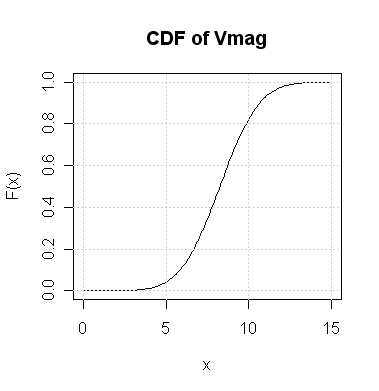
| Example:
Suppose that I choose a random star from the Hipparcos data
set. If I tell you that its Vmag is a random variable
with the following CDF then what is the chance that it takes values
≤ 10? Also find out the value x such that
the chance of Vmag being ≤ x is 0.4.
For the first question the required probability is F(10)
which, according to the
graph, is slightly above 0.8.
In the second part we need F(x) = 0.4. From the graph it
seems to be about 7.5.
Just to make sure that these are indeed meaningful, let us load
the Hipparcos data set and check:
hip = read.table("HIP.dat", header = TRUE, fill = TRUE)
attach(hip)
n = length(Vmag) #total number of cases
count = sum(Vmag<=10) #how many <= 10
count/n #should be slightly above 0.8
This checks the answer of the first problem. For the second
count = sum(Vmag<=7.5) #how many <= 7.5
count/n #should be around 0.4
|
So you see how powerful a CDF is: in a sense it stores as much
information as the entire Vmag data. It is a
common practice in statistics to regard the distribution as the
ultimate truth behind the data. We want to infer about the
underlying distribution based on the data. When we look at a data
set we actually try to look at the underlying distribution
through the data set!
R has many standard distributions already built into it. This
basically means that R has functions to compute their CDFs.
These functions all start with the letter p.
| Example:
A random variable has standard Gaussian distribution. We know
that R computes its CDF using the function pnorm. How to
find the probability that the random variable takes values
≤ 1?
The answer may be found as follows:
pnorm(1)
|
For every p-function there is a
q-function that is basically its inverse.
| Example:
A random variable has standard Gaussian distribution. Find
x such that the random variable is ≤ x with
chance 0.3.
Now we shall use the function qnorm:
qnorm(0.3)
|
OK, now that we are through our little theory session, we are
ready for the nonparametric lab.
One sample nonparametric tests
Sign-test
In a sense this is the simplest possible of all tests. Here
we shall consider the data set LMC.dat that stores the measured
distances to the Large Magellanic Cloud. (As always, you'll need
to save the file on your desktop.)
LMC = read.table("LMC.dat",head=T)
data = LMC[,2] #These are the measurements
data
We want to test if the
measurements exceed 18.41 on an average. Now, this does
not
mean whether the average of the data exceeds 18.41, which is trivial
to find out. The question here is actually about the underlying
distribution. We want to know if the median of the underlying
distribution exceeds 18.41, which is a less trivial question,
since we are not given that distribution.
We shall use the sign test to see if the median is 18.41 or larger.
First it finds how many of the
observations are above this value:
abv = sum(data>18.41)
abv
Clearly, if this number is large, then we should think that the
median (of the underlying distribution) exceeds 18.41. The
question is how large is ``large
enough''? For this we consult the binomial distribution to get
the p-value. The rationale behind this should come from
the theory class.
n = nrow(LMC)
pValue = 1-pbinom(abv-1,n,0.5)
pValue
We shall learn more about p-values in a later
tutorial. For now, we shall use the following rule of thumb:
If this p-value is below 0.05, say, we shall conclude that
the median is indeed larger than 18.41.
Wilcoxon's Signed Rank Test
As you should already know from the theoretical class, there is a
test called Wilcoxon's Signed Rank test that is better (if a little
more complicated) than the sign test. R provides the function
wilcox.test for this purpose. We shall work with the
Hipparcos data set this time, which we have already loaded.
We want to see if the median of the distribution of the
pmRA variable is 0 or not.
wilcox.test(pmRA, mu=0)
Since the p-value is pretty large (above 0.05, say) we
shal conclude that the median is indeed equal to 0. R itself
has come to the same conclusion.
Incidentally, there is a little caveat. For Wilcoxon's Rank Sum Test
to be applicable we need the underlying distribution to be
symmetric around the median. To get an idea about this we should
draw the histogram.
hist(pmRA)
Well, it looks pretty symmetric (around a center line).
But would you apply Wilcoxon's
Rank Sum Test to the variable DE?
hist(DE)
No, this is not at all symmetric!
Two-sample nonparametric tests
Here we shall be taking about the shape of distributions. Let us
first make sure of this concept. Suppose that I make a list of
all the people in a capitalist country
and make a histogram of their incomes.
I should get a histogram like this
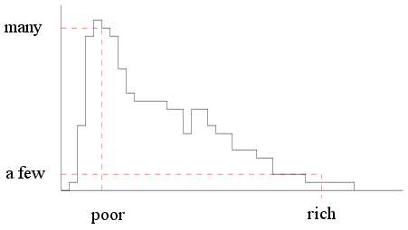 |
| Income histogram of a capitalist
country |
But if the same thing is done for a socialist country we shall
see something like this (where almost everybody is in the middle
income group).
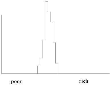 |
| Income histogram of a socialist
country |
Clearly, the shapes of the histograms differ for the two
populations. We must be careful about the term ``shape'' here. For
example, the following two histograms are for two capitalist
countries, one rich the other poor.
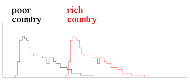 |
| Income histograms two capitalist
countries |
Here the histograms have the same shape but differ in
location. You can get one from the other by applying a
shift in the location.
This is a very common phenomenon in statistics. If we have two
populations with comparable structure they often have similar
shapes, and differ in just a location shift. In such a situation
we are interested in knowing about the amount of shift. if the
amount of shift is zero, then the two populations behave
identically.
Wilcoxon's rank sum test is one method to learn about the amount
of shift based on samples from the two populations.
We shall start with the example done in the theory class, where
we had two samples
x = c(37,49,55,57)
y = c(23,31,46)
m = length(x)
n = length(y)
We are told that both the samples come from populations with the
same shape, though one may be a shifted version of the
other.
Our aim is to check if indeed there is any shift or not.
We shall consider the pooled data (i.e., all the 7 numbers
taken together) and rank them
pool = c(x,y)
pool
r = rank(pool)
r
The first m=4 of these ranks are for the first
sample. Let us
sum them:
H = sum(r[1:m])
H
If the the two distributions are really identical (i.e.,
if there is no shift) then we should have (according to the
theory class) H close to the value
m*(m+n+1)/2 #Remember: * means multiplication
Can the H that we computed from our data be considered
``close enough" to this value? We shall let us R determine that
for us.
wilcox.test(x,y)
So R clearly tells us that there is a shift in location. The
output also mentions a W and a
p-value.
tutorial. But W is essentially what we had called
H. Well, H was 21, while W is 11. This
is because R has the habit of subtracting
m(m+1)/2
from H and calling it W. Indeed for our data set
m(m+1)/2 = 10,
which perfectly accounts for the difference between our H
and R's W.
You may recall from the theory class that H is called
Wilcoxon's rank sum statistic, while W is the Mann-Whitney
statistic (denoted by U in class).
Now that R has told us that there is a shift, we should demand to
estimate the amount of shift.
wilcox.test(x,y,conf.int=T)
The output gives two different forms of estimates. It
gives a single value (a point estimate) which is 16.
Before it gives a 95% confidence interval: -9 to
34.
This
basically means that
we can say with 95% confidence that
the true value of the shift is between -9 and 34.
We shall talk more about confidence intervals later. For now let
us see how R got the poit estimate 16. It used the so-called
Hodges-Lehman formula, that we have seen in the theoretical
class. To see how this method works we shall first form the following
"difference table"
  | 23 31 46
------------
37| 14  6 -9
49| 26 18  3
55| 32 24  9
57| 34 26 11
Here the rows are headed by the first sample, and columns by the
second sample. Each entry is obtained by subtracting the column
heading from
the row heading (e.g., -9 = 37-46). This table, by the
way, can be created very easily with the function outer.
outer(x,y,"-")
|
| | |
|
The outer function is a very useful (and somewhat
tricky!) tool in R. It takes two vectors x, and y,
say, and some function f(x,y). Then it computes a matrix
where the (i,j)-th entry is
f(x[i],y[j]).
| |
| | |
|
Now we take the median of all the entries in the table:
median(outer(x,y,"-"))
This gives us the Hodges-Lehman estimate of the location shift.