Organisation and dynamics of surface magnetic field

Magneto-convective processes in the photospheric and sub-photospheric layers of the Sun play crucial roles in the magnetic structuring and dynamics of upper atmospheric layers. The near-surface layers are the regions where the plasma β (= the ratio of gas to magnetic pressure) transitions from β>>1 in the interior to β<<1 in the outer atmospheric layers. The β~1 photospheric boundary layer is also the region where the continuum optical depth τc~1, which separates the optically thick interior from the thin outer atmosphere. Hence, this boundary layer is subject to a strong coupling of very different scales of dynamical interests, and is difficult to study both observationally and theoretically.

Both very fast imaging and fast spectroscopic measurements are necessary to study the highly complex processes in this region. Spectropolarimetry, the study of Stokes vectors (Polarization) of a spectral line to infer physical conditions prevailing in a dynamic magnetized medium is the most sensitive tool that is available.

Flux emergence and active region dynamics

Emerging magnetic flux through the β~1 layers expand and merge above a certain height called the "magnetic canopy height" and fill the available space in the β<<1 region. Below the photosphere, due to the dominant gas pressure forces, the magnetic fluxes are passive and are confined to individual and separated flux tubes. The emergence from below is, thus, in the form of individual flux tubes, which are expected to carryoppositely directed currents on either side of the flux tube boundaries as well as twists.

Measurements of currents and twists in emerging flux tubes is important both to infer the dynamical evolution of the magnetic flux tubes while they rise through the solar interior to the surface as well as to understand the role of the twist leading to instabilities and eventual dissipation of magnetic energy in the solar atmosphere. Studies of helicity and energy fluxes in active regions (e.g. Ravindra et al., 2008) give important insights into the coronal dynamics and activity.

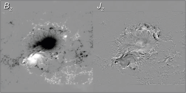
Figure 2 Line of sight magnetogram Bz (on the left), and the derived current Jz = Curl Bz map (on the right), of active region NOAA 10930 observed by HINODE SP/SOT on December 12, 2006 (Courtesy: M. DeRosa, Lockheed-Martin Solar and Asrophysics Lab).

Present vector magnetograms show a persistent pattern of electric currents (see Figure 2) and helicity associated with strong magnetic fields of active regions. NLST will be able to address the following questions: (1) how are the electric currents in the emerging flux tubes structured and how do they interact with the current systems already developed in the overlying canopy fields?; (2) what are the basic mechanisms of flux submergence?; (3) how does the magnetic helicity interact with mass flows down the legs of raising flux tubes and how does it affect the overall helicity flux into the upper atmosphere?; and (4) what are the dynamical consequences of helicity driven vortical flows in the photosphere?.

Dynamical evolution of small-scale magnetic field

Extensive theoretical and numerical studies (Parker 1978, Spruit and Zweibel 1979, Spruit 1979, Hasan 1984, Venkatakrishnan 1986, Rajaguru and Hasan 2000) as well as 2- and 3-D MHD simulations (Nordlund 1985, Steiner 1999) have shown that there are two important processes in action in the formation, organisation and stabilization of small-scale strong magnetic flux tubes that dot the super-granular boundaries. They are flux expulsion and convective collapse. While the existence of the former process, viz. flux expulsion, finds easy confirmation through the established pattern of magnetic flux residing in the convective down flow regions, observational evidence for the latter process is very challenging to establish. This is due to the fact this process happens very fast and over a small spatial scale. Though recent high resolution observations from HINODE have provided evidences, a routine mapping of this process so as to be able to study it statistically and test theoretical predictions requires high sensitivity and high cadence polarimetric observations.

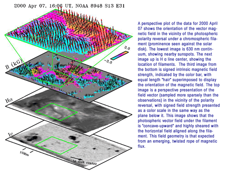
Figure 3 Observations of different layers of Sun using different instruments leading to inference of vector magnetic field maps. The continuum intensity (bottom-most), with H-alpha above it, and inferred vector magnetic field and a blow up of a small region are shown at higher stacks (Courtesy:Lites 2005).

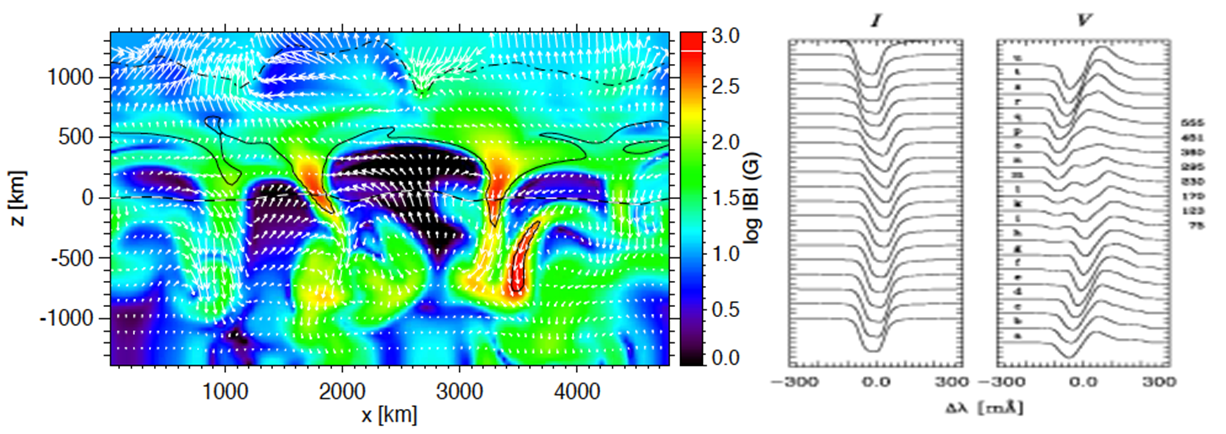
Figure 4 Numerical simulations predict how magnetic flux tubes dynamically interact with convection to produce MHD waves and shocks that drive heating and upward ejection of material in the overlying atmosphere. Radiative transfer calculations (right panel) predict the evolution of Stokes I and V profiles (Courtesy:O. Steiner, 2007).

Observations of different layers of Sun using different instruments leading to inference of vector magnetic field maps is shown in Figure 3.5. This figure shows that multi wavelength observations are needed to map vector magnetic fields at different heights in solar atmosphere. NLST will provide an opportunity to undertake such observations. High resolution numerical simulations leading to MHD waves and corresponding Stokes vector calculations are routinely made these days (Figure 4). They will need high resolution observations for validating purposes. Small scale features can be easily identified with high resolution. NLST instruments, with adaptive optics, will test the presence and efficiency of the convective collapse mechanism by both spatially and temporally resolving it in action.

The kilo Gauss strength network elements provide mechanical and energetic coupling between the photospheric, chromospheric and higher layers through waves as well as through associated shock dynamics related transients such as jets, coronal bright points, blinkers etc. This makes solar atmosphere highly dynamic. These strong flux concentrations constantly undergo buffeting by the granular flows reaching speeds of 1-5 km/s. Observations of these structures require high time cadence with fast cameras.

Spectropolarimetry and 3-D structure of sunspots and magneto-convection

Sunspots are classic examples that portray the complexity and rich physics that magnetohydrodynamic phenomena exhibit on stellar surfaces. Despite several centuries of observations and intense study, we still lack a consistent scientific explanation of the observed nature of a sunspot (Solanki, 2003). The way they remain stable and survive over a month in a turbulent environment continues to be a puzzle. Understanding what drives the radial Evershed flow in the penumbra of a sunspot is still a challenging problem.

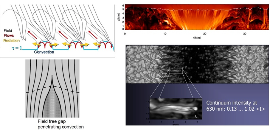
Figure 5 A 3D nonlinear magnetoconvection simulation of a sunspot with Evershed flows by M. Rempel et al. The left panels depict the geometry of magnetic and flow fields facilitating the magnetoconvection interactions as seen in the simulations, snapshots of which are in the right panels: the top right panel shows the magnetic field strength, varying from zero (dark) to about 9000 Gauss (white shade), and the bottom right panel shows a continuum intensity snapshot.(Courtesy: O. Steiner, 2007).

We are currently in a period of revived attention mostly fuelled by our increased numerical computational capabilities to simulate MHD processes. These observed features are indicative of a modified pattern of convection. However, identifying and understanding the exact physical causes and mechanisms behind these complex magneto-convective processes require solving the full 3-D MHD equations.

With prescribed magnetic field geometries representative of sunspot like situations, modelers have performed 3D nonlinear simulations of interactions between turbulent convection and magnetic fields, thereby obtaining a new magneto-convective origin for the Evershed flows (Scharmer et al., 2008, Rempel and Schussler, 2008). Here, the convective interactions between an upward hot plume and magnetic field produce all the necessary ingredients to drive a horizontal Evershed flows depicted in Figure 5.